찾으시는 정보가 있으시다면
주제별reference를 이용하시거나
우측 상단에 있는 검색기능을 이용해주세요

Numpy Random

Random number doesn’t mean a different number every time

Random means something that can’t be predicted logically

Pseudo Random

Programs are definitive set of instructions

It means there must be some algorithm to generate a random number as well

Thus it is not truly random, is called pseudo random

True Random

In order to generate a truly random number on our computers we need to get the random data from some outside source

• Is generally our keystrokes, mouse movements, data on network etc.

from numpy import random

a = random.randint(100)	# output random integer from 0 to 100
b = random.rand()		# output random float from 0 to 1
c = random.randint(100, size=(5))	# output 1-D array containing 5 random integers from 0 to 100
d = random.randint(100, size=(3,5))	# output 2-D array containing 3*5 random integers from 0 to 100
e = random.rand(3,5)		# output 2-D array containing 3*5 random float from 0 to 1
arr = [1,2,3,4,5]
f = random.choice(arr)	# output Random value based on an array of values
g = random.choice(arr, size=(3,5))	# output 3*5 Random value based on an array of values
# To specify the probability for each value
h = random.choice(arr, p=[0.1, 0.3, 0.4, 0.2, 0.0])	# output random integers based on an array of values, the value 5 will never occur

Permutation

from numpy import random
import numpy as np
arr = np.array([1,2,3,4,5])

# Changing arrangement of elements in-place
random.shuffle(arr)
print(arr)

# Returns a re-arranged array(and leaves the original array un-changed)
print(random.permutation(arr))

Seaborn

Is a libarary that uses Matplotlib underneath to plot graphs

• It will be used to visualize random distributions

distplots

• It stands for distribution plot, it takes as input an array and plots a curve corresponding to the distribution of points in the array

Distribution

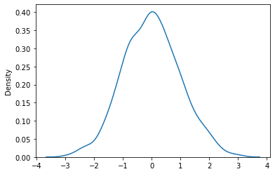
Normal

Is called the Gaussian Distribution

It has 3 parameters

• loc : Mean, where the peak of the bell exits

• scale : Standard deviation, how flat the graph distribution should be

• size : The shape of the returned array

The curve of a normal distribution is also known as the Bell Curve because of the bell-shaped curve

from numpy import random
import matplotlib.pyplot as plt
import seaborn as sns

sns.distplot(random.normal(size=1000), hist=False)
plt.show()

Binomial

Is a Discrete Distribution

It describes the outcome of binary scenarios

It has 3 parameters

• n : number of trials

• p : probability of occurrence of each trial(e.g. for toss of a coin 0.5 each)

• size : The shape of the returned array

from numpy import random
import matplotlib.pyplot as plt
import seaborn as sns

sns.distplot(random.normal(loc=50, scale=5, size=1000), hist=False, label= ‘normal’)
sns.distplot(random.binomial(n=100,p=0.5,size=1000), hist=False, label= ‘binomial’)
plt.show()

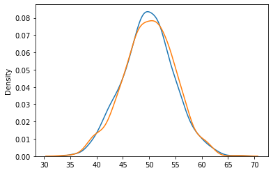
Difference between Normal and Binomial Distribution

• Main difference is that normal distribution is continuous whereas binomial is discrete, but if there are enough data points it will be quite similar to normal distribution with certain loc and scale

Poisson

Is a Discrete Distribution

It estimates how many times an event can happen in a specified time

It has 2 parameters

• lam : rate or known number of occurrences e.g. 2 for above problem

• size : the shape of the returned array

from numpy import random
import matplotlib.pyplot as plt
import seaborn as sns

sns.distplot(random.normal(loc=50, scale=7, size=1000), hist=False, label= ‘normal’)
sns.distplot(random.poisson(lam=50, size=1000), hist=False, label= ‘poisson’)
sns.distplot(random.binomial(n=1000, p=0.05, size=1000), hist=False, label= ‘binomial’)

plt.show()

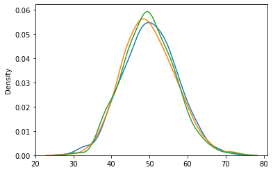
Difference Between Normal and Poisson Distribution

• Normal distribution is continuous whereas poisson is discrete

Differnece Between Poisson and Binomial Distribution

• Is very subtle it is that, binomial distribution is for discrete trials, whereas poisson distribution is for continuous trials

• But for very large n and near-zero p binomial is near identical to poisson such that n*p is nearly equal to lam

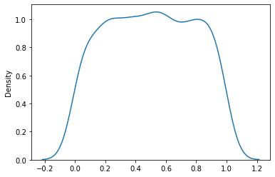
Uniform

Used to describe probability where every event has equal chances of occurring

It has 3 parameters

• a : lower bound, default 0

• b : upper bound, default 1

• size : the shape of the returned array

from numpy import random
import matplotlib.pyplot as plt
import seaborn as sns

sns.distplot(random.uniform(size=1000), hist=False)
plt.show()

Logistic

Is used to describe growth

Used extensively in machine learning in logistic regression, neural networks etc.

It has 3 parameters

• loc : mean, where the peak is, default 0

• scale : standard deviation, the flatness of distribution, default 1

• size : the shape of the returned array

     from numpy import random
     import matplotlib.pyplot as plt
     import seaborn as sns
     sns.distplot(random.logistic(size=1000),hist=False)
     plt.show()

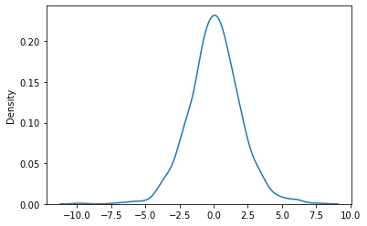
Difference Between Logistic and Normal Distribution

• Both are near identical, but logistic has more area under the tails

• It representage more possibility of occurrence of an events further away from mean

Multinomial

Is a generalization of binomial distribution

It describes outcomes of multi-nomial scenarios unlike binomial where scenarios must be only one of two

It has 3 parameters

• n : number of possible outcomes

• pvals : list of probabilities of outcomes

• size : the shape of the returned array

from numpy import random
x = random.multinomial(n=6,pvals=[1/6,1/6,1/6,1/6,1/6,1/6])

As they are generalization of binomial distribution their visual representation and similarity of normal distribution is same as that of multiple binomial distributions

Exponential

Is used for describing time till next event

It has 2 parameters

• scale : inverse of rate, default 1

• size : the shape of the returned array

from numpy import random
import matplotlib.pyplot as plt
import seaborn as sns

sns.distplot(random.exponential(size=1000), hist=False)
plt.show()

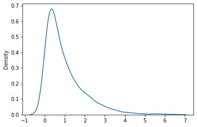
Relation Between Poisson and Exponential

• Poisson distribution deals with number of occurences of an event in a time period whereas exponential deals with the time between these events

Chi Square

Is used as a basis to verify the hypothesis

Is has 2 parameters

• df : degree of freedom

• size : the shape of the returned array

from numpy import random
import matplotlib.pyplot as plt
import seaborn as sns

sns.distplot(random.chisquare(df=1,size=1000),hist=False)
plt.show()

Rayleigh

Is used in signal processing

It has two parameters

• scale : decides how flat the distribution will be default 1

• size : the shape of the returned array

from numpy import random
import matplotlib.pyplot as plt
import seaborn as sns

sns.distplot(random.rayleigh(size=1000),hist=False)
plt.show()

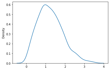
Similar Between Rayleigh and Chi Square Distribution

• At unit stddev the and 2 degrees of freedom Rayleigh and chi square represent the same distributions

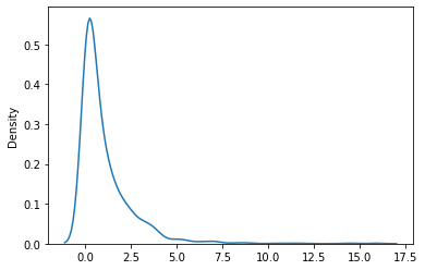
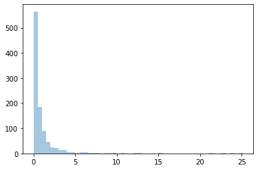
Pareto

80 - 20 distribution (20% factors cause 80% outcome)

It has 2 parameters

• a : shape parameter

• size : the shape of the returned array

from numpy import random
import matplotlib.pyplot as plt
import seaborn as sns

sns.distplot(random.pareto(a=2, size=1000),kde=False)
plt.show()

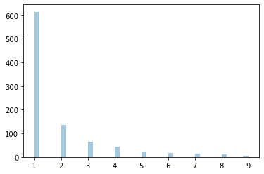
Zipf

Are used to sample data based on zipf’s law

• Zipf’s law : In a collection the nth common term is 1/n times of the most common term

It has 2 parameters

• a : distribution parameter

• size : the shape of the returned array

from numpy import random
import matplotlib.pyplot as plt
import seaborn as sns

x = random.zipf(a=2, size=1000)
sns.distplot(x[x<10], kde=False)
plt.show()